Week 5 Lex 3: Electrostatics in Material Media. ( Dielectrics)

Having covered a number of issues for Electrostatics in free space we now move to the study of Electrostatics in a material media like dielectrics/insulators. The basic difference with conductors in this case is that in a dielectric charges have restricted mobility unlike free charges in a conductor. So the charges cannot move freely but they can be displaced a little from their equilibrium position
which makes the atom neutral.


When a dielectric material is placed in an external electric field a separation of the +ve and -ve charges take place so that there is a field inside the dielectric material which opposes the external field such that the net field inside is reduced. Due to the charge separation surface charges appear on the dielectric.


At the microscopic level the centers of the +ve and -ve atomic chrage distributions are displaced by the external applied field ( like the problem of two spherical charge distributions +ρ and -ρ displaced by a small distance d done in a DIPA). The atom is now said to be polarized and develops a small dipole moment p which is proportional to the applied field E such that p=α E and α is called the atomic polarisability. For a molecule the situation is more complex but once more a dipole moment develops but the polarisability α is now direction dependent and is a rank 2 tensor.


Apart from this certain molecules due to their asymmetric structures have a charge distributions with a FROZEN-IN PERMANENT dipole moment p. These are called POLAR molecules. In an uniform external field E these permanent dipoles feel a torque N=p X E which tends to orient the dipole moment vector in the direction of the external field ( for a non uniform field the dipole experiences a force F=(p.∇) E. Note that (p.∇)is a scalar differential operator which operates on each component of the vector field E. This is the operator version of scalar multiplication of a vector.)


So the microscopic picture that emerges for a dielectric from the above consideration is that a dielectric material either develops induced dipoles or has permanent dipoles ( for polar molecules)
both of which tend to orient along the direction of the applied external field. Some of this orientation will even stay after the field is removed especially for Polar molecules. So in a dielectric material
we have a large number of dipoles oriented in the same direction. This results in a dipole moment per unit volume which is called the Polarization vector P .


Now it is possible to calculate the field due to such a Polarised material by finding the Potential due to a small volume dτ' which has a dipole moment Pdτ' and integrating over the entire volume. Manipulation of this volume integral using product rules and the Divergence theorem show that the potential at some point due to a Polarized material is due to two contributions.

(i) A surface BOUND chrage density σ_b=P. n cap
(ii) A volume BOUND charge density ρ_b=-∇. P


This mathematical result is confirmed by a physical analysis of the microscopic dipoles canceling each other in the volume resulting in a surface bound charge density and a volume bound charge density when the cancellations are not complete in the volume due to unequal dipoles ( non constant dipole moment /unit volume which is non uniform Polarisation). The expression match exactly confirming the mathematical analysis using Vector Calculus.

Week 5 Lex 2: The Method of Images.

The method of images for electrostatic problems is a way to obtain the potential V for a problem by identifying it with the known ( simpler to calculate) potential V of a different electrostatic problem but satisfying the same boundary condition as the original V in the region of interest. Uniqueness theorem then ensures that the two potentials are identical in the region of interest.


Classic Image Problem I:


A point Charge q placed at a distnace d in front of an infinite conducting plane which is grounded, to find the potential at a point above the plane.


The trick to solve this problem is to identify that one of the equipotential at the mid point between two equal and opposite charge +q and -q is a plane and its at V=0. This is identical to the case of a point charge in front of a conducting plane at ZERO potential because the potential satisfies the same boundary conditions V=0 at z=0 taking the z-axis to be perpendicular to the plane.


Thus the image problem is that of two charges +q and -q situated at equal distance from the origin in the +ve and -ve direction of the z-axis. Now the potential due to this arrangement is very simple to calculate by superposition of the potential due to each of the two charges the image charge and the point charge.


Note that the solution is only valid above the conducting plane. Below the plane the situation is completely different but that is excluded from our region of interest. Uniqueness theorem ensures that in the region of interest this is the only UNIQUE solution that satisfies the given boundary conditions. Hence the solution for the potential


Note also that the image charge cannot be placed in the region of interest because that would completely change the original problem we are seeking a solution to. Its important to understand that the method of images is a method to find an alternate simple problem whose potential is identical with that of the original problem due to both satisfying the same boundary conditions in the region of interest.


The solution can be easily extended to that of the isolated  ( ungrounded ) conducting plane.


Classic Image Problem II:


A point charge q is placed outside at the distance a from the center of a conducting sphere of radius Rwhich is grounded, to find the potential everywhere outside. The trick for this is to identify that one of the equipotentials for a system of two unequal charges q and q' is a sphere. So the only thing now is to set the boundary conditions.
Since the original sphere is grounded ( at ZERO potential) in the new problem we will have to adjust q' so that the spherical surface is at V=0. Now its esay to calculate V ( IPSA Problem) for the two unequal charges and see that the image charge must be set at x=R²/a from the center and its magnitude should be q'=-R/a x q to make the potential V(R)=0.


The problem with the grounded sphere may easily be extended to cover an isolated ( ungrounded) sphere. The sphere would be an equipotential now at V=V₀


It is now possible to use these two image problems and superposition of potentials to solve more complex problems which I have mentioned in the lecture and some of which will be discussed in the future tutorials.

Week 5 Lex 1: Uniqueness Theorem and Electrostatic Boundary Conditions

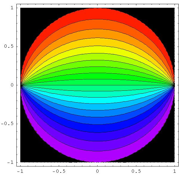
The contour map of the solution to Laplace's equation inside the disk. (Courtesy http://oak.ucc.nau.edu/jws8/classes/461.2009.7/animations.html and Google).

Having seen the multipole expansion as a method to obtain the approximate potential

far away from a localized charge distribution we now look for other methods to obtian the potential exactly. The most direct method is to solve the Laplace or Poisson equation ∇² V=0 or ∇² V= -ρ/ε₀ as the case may be to obtain the poetntial V. However its not easy to solve these equations as they are partial differential equations ( PDE) and also they have infinite number of solutions. The solution specific to a problem is obtianed by using boundary conditions ( values of potential at boundaries, which are determined from the physics of the problem. The Uniqueness theoerm pertains to such boundary conditions and the uniqueness of a solution which satisfies a specific set of boundary conditions.

Solutions to the Laplace equations are called harmonic functions and they have certain special properties.

(i) The value of the potential V(r) at a point r is given by the average of the poetntial over a sphere S of radius R with the pint r as its center.

(ii) Follows from (i) There cannot be any local maxima or minima of V, all extremum values of V occur at the boundaries. ( This is obvious because if V had a maxima

its value would be higher than on a sphere of radius R and hence cannot be the average V over that sphere. Average value can neither be larger nor smaller than the

largest and smallest values in the sample over which the average is being taken. It must lie somewhere in between.)

Proof: Take a point charge q outside a spherical surface of radius R. Its easy to show that the average potential over the surface S is equal to the potential produced

at the center. By superposition this can be extended for any arbitrary discrete or continuous charge distributions outside S, For all such configurations the average potential over the sphere is equal to the net potential produced at the center of S

First Uniqueness Theorem: The solution to the Laplace equation in a volume τ is uniquely determined if the potential V is specified at all boundary surfaces

S.

Proof: Assume two solutions V₁ and V₂ which staisfy the Laplace equation in τ and which have the same value V_S at S. Its easy to see that V₃=V₂ -V₁ also satisfies the Laplace equation and its value is ZERO on S. Since for Laplace equation all extrema must occur at the boundary so the value ZERO is both maxima and minima for V₃.

Which implies that V₃=0 everywhere. So V₂-V₁=0 so

V₂=V₁. So V is unique. this can be easily extended to regions with a non zero charge distribution ρ also by using the Poisson equation.

Corollary: The potential in a volume τ is UNIQUELY determined if the charge density is specified throughout and the potential V is specified on all boundaries

S.

The second Uniqueness Theorem is for conductors and is stated as ; In a  volume τ surrounded by conductors and having a specified chrage density ρ the electric field E is UNIQUELY determined if the total charge Q on each conductor is given. ( Proof: Read from Griffiths).

Electrostatic boundary conditions: The normal component of the electric field is discontinuous across any boundary with a charge distribution σ by an amount σ / ε₀.

The tangential component of the electric field is always continuous across any boundary.

The potential V is always continuous across any boundary but its derivatives are not. In particular the normal derivative ∂ V/∂ n cap =∇ V. $n$ cap is discontinuous by -(σ/ε₀)

A Guide to Preparations.

Dear Students,

I am getting a lot of queries about Mid Sem I. So here is a guide to
preparations. This is only a guide.

1. Dont panic or be stressed. It is never helpful. If you need help
please call the exam helplines ( this will be sent by DOAA) or talk to
your student counsellor.

2. Study the class notes with Griffiths text and clarify all the concepts.
Work out fully all the DIPA and IPSA Problems. Mid Sems will be of the
level of DIPA problems and some short questions both problems and
concepts. There will be no long theoretical questions like derivations.

3. You can try other problems of same level in Griffiths but very
complicated and hard problems are not necessary to be done. Griffiths has
many problems and you should refer to only what I have taught. Everything
in Griffiths is not in the syllabus.

4. I have already announced in class that long expressions for operators
in curvilinear coordinates will be supplied. You dont have to memorize them.
You should know how to use and manipulate them as in the DIPA and IPSA
problems. ( The general derivation is in Appendix A of Griffiths, but that
is only for your interest. Its not included in the syllabus.)

5. Complicated problems with delta function and its properties will not be
asked. Only the problems of the same level as in IPSA and DIPA.

6. It will be useful ( time saving) to remember some standard
expressions/formula for potentials and fields of standard configurations.
Anything that has been derived/worked out in the class or DIPA or IPSA can
be used directly.

6. IMPORTANT: Please take some time to read and understand the question.
Many times people misread the question and then their answers are
completely incorrect. You will have to answer only what has been asked.


I hope this will help.

Best of luck

GS

DIPA SET 4 PDF FILE IN YOUR E-MAIL BOXES.

Please note that DIPA Set 4 PDF file is in your e-mail.

Week 4 Lex 3: Multipole Expansion II

The multipole expansion arises from the idea that the potential due to a point charge q at a distance r goes as 1/r. If we calculate the approximate potential at a large distance from a physical dipole which is a pair of equal and opposite charges +q and -q at a distance d  where the vector d is from the -ve to the +ve charge is given by a binomial expansion to first order ( higher orders neglected) as 
V=(1/4πε₀)[ q d cos θ/r²] and goes as 1/r² to a first order.


This tells us that it may be possible to obtain the approximate potential at a large distance from an arbitrary charge configuration in terms of a series of contributions in powers of (1/r). This is somewhat like expressing a complex waveform in terms of some simple waves of different frequencies ( fundamentals and harmonics), called a Fourier expansion.. What allows this is the Superposition Principle.


When we expand the denominator of the the expression for the potential at a faraway point r due to an arbitrary volume charge distribution ρ(r') given as
V=(1/4πε₀)∫_τ ρ(r')dτ'/r
( note that r is the Griffiths script/curly r. )
in a binomial expansion, we obtain a series of contributions in powers of (1/r) which is the distance between the source point r' and the field point r. The coefficient of each power of (1/r) is an integral that provides the respective moments like the monopole moment ( total charge Q=∫ ρ(r')dτ') then a dipole moment p= ∫_τ r'ρ(r')dτ' and
the contribution to the potential is given as V_dip=(1/4πε₀)p. r cap /r² please note that r cap is a unit vector along r. Note that θ or θ' is simply the angle between the position vectors r and r'. It is not the polar angle unless z axis is chosen along the r' or r direction. Note that this is the dipole moment of a PURE DIPOLE


*For a point charge at origin the monopole term is the only non zero term and the potential due to a point charge is EXACT all higher multipoles vanishing. ( Check it out)


*The dipole moment expression works for a line charge λ, surface charge σ distribution replacing the volume distribution ρ and integrating over
a surface or a line.


For a discrete point charge distribution of q_i at r'_i the pure dipole moment is p=∑_i=1ⁿ q_i r'_i. A physical dipole moment is a special case of this for just two charges +q and -q and is given as p=qd where the vector d is the vector from - to the + charge. This is consistent as it gives the correct potential where
for a physical dipole. But note that this potential is approximate because for a physical dipole of two unlike but equal charges the monopole term is zero as total charge Q=0 but higher multipole terms are not zero. They are smaller than the dipole contribution and hence neglected in the approximation that the field point r is far away from the source.


It should be obvious now that for a single point charge away from the origin ( that is r' not equal to 0) will have all possible moments starting from the monopole moment ( total charge Q=q in this case) and all possible such terms in the expression for the potential V at a field point r.


* The physical dipole reduces to a pure dipole in the limit q
goes to infinity and d goes to 0 with qd=p held fixed. So a physical dipole are finitely separated charges and a pure dipole is more like a point. The pure dipole is the second moment in the multipole expansion. For large distances the field
of a pure dipole and a physical dipole are identical but are very different close to the source. ( See the two figures given in Griffiths).


The multipole expansion is dependent obviously on the coordinate system. The example of a point charge q away from the origin is an example of this where all higher multipoles also contribute although the dominant term is the monopole moment.


For a shift in origin the monopole moment Q does not change. The (pure) dipole moment changes due to the shift except when the total charge Q=0 ( algebraic sum). In that case ( for total charge Q=0) the (pure) dipole moment is unchanged. See the example for a shift of origin by a vector a  in Griffiths at the end of the section which was discussed in class.

For quick reference

http://cr4.globalspec.com/blogentry/2842/Multipole-Expansion

Week 4 Lex 2: Conductors and Multipole Expansion.

Conductors: In this lecture we first examine the issue of charged and uncharged conductors in an electric field. A perfect ideal conductor is characterized by an unlimited supply of free electrons. When a conductor is placed in an external electric field E ₀ the electrons which are very loosely bound to the atom flow in the direction opposite to that of the external electric field. This causes separation of the positive and negative charges within the conductor and this sets up an induced Electric field E_ind inside the conductor in opposition to that of the external field. The charges flow till the induced field completely cancels the external applied field inside the conductor. Hence the field inside a conductor is ZERO and all charges appear on the surface of the conductor. ( inside the conductor the charge density is ZERO. This is because if any chrage density builds up inside the conductor, the resultant electric field with drive the charges till the density will is zero.)


Since the field is zero and the field is derivative of the potential E=-∇V so the conductor must be an equipotential surface with a constant potential that extends into the conductor. So on the surface of the conductor and inside the potential is constant. This also shows that the electric field has a discontinuity ( increases to a finite value from zero discontinuously) just away from the surface of the conductor. This always happens whenever the electric field encounters a surface charge density.


Now since dV=∇V.dl=0 on the surface as V is constant on the surface, this shows that the electric field just away from the surface of a conductor is normal to the surface ( -∇V is perpendicular to dl on the surface to make dV=0 on the surface which is an
equipotential).


So whenever a charge q is brought near a conductor the electric field draws the electrons to the side closer to the charge leaving the positive charges piled up on the side which is further away. Hence an induced charge distribution occurs on the surface of the conductor due to the presence of the charge q. As the conductor was originally neutral and since the field inside the conductor is zero, application of Gauss theorem shows that the induced surface charge is always equal to -q.


The fact that a conducting surface is an equipotential is used in a Capacitor which is an arrangement of two or more conductors at different potentials with charges +Q and -Q. The charge Q=CV where C is the capacitance of the arrangement. Note that the
capacitance is a geometrical quantity and depends on the shape size and arrangement of the conductors. The Capacitor when charged by a battery has electrons removed from the +ve plate to the -ve plate and this process continues till the electric field due to the plate charges exactly balances the electric field due to the battery. The work done to move the electrons is stored in the capacitor electrostatic (potential) energy. This energy will appear when the conductors are shorted through sparking. The energy expression may be calculated and W=1/2CV²


Multipole Expansion: In what we have seen over the last 3 weeks it seems that the fundamental problem of electrostatics which was to find the electric field due to a certain charge
distribution/configuration is far easier to obtain provided we know the potential due to this charge distribution at the field point since E=-∇ V and differentiation is easier than integration. However its not easy to find the potential due to a charge distribution because that also involves solving an integral although the integrand in this case is a scalar. Although possible in simple cases its not easy to do this integral for an arbitrary chrage distribution.


The multipole expansion is a way around this difficulty to obtain at least the approximate potential at a field point far way from the charge distribution. We will see that the approximate potential is a very good estimate and becomes better as more and more terms in the expansion ( series) are considered.


A single point charge is called a monopole and we know the potential due to this. A simple binomial expansion provides us with the approximate potential due to a charge pair called a physical dipole. This provides us with the idea of expanding the potential due an arbitrary localized charge distribution at a field point far away from the charge configuration. A binomial expansion an the approximation that the point at which the potential is required is far away provides us with a systematic expansion of the potential V(r) in terms of a series in powers of (1/r) and specific basic charge configurations like a monopole, dipole, quadrupole, octupole etc. The approximation becomes better and better as more terms in the series are included. Note that each successive term contributes less and less to the potential as powers of (1/r). Schematically the series may be written as
V(r)=1/4πε₀ [ K₀/r + K₁/r ² + K₂/r ³ +...........]
Where the terms denote the monopole, dipole and quadrupole contributions respectively. Note that the dipole term in the monopole expansion is different from the potential due to a physical dipole.
We will have more to say about this in the next lecture.

Week 4 Lex 1: Work and Energy in Electrostatics.

The picture is that of a Plasma Lamp that works using Electrostatic
charges.

After having looked at the Laplace and Poisson equations satisfied by the electrostatic potential V (note that V is scalar field) in this week we start with issues of work and energy in electrostatics.

Since the Curl E of the electric field is zero the field E =-∇ V. This means that the electrotstatic filed is a conservative field and the work done ( which is the line integral of the force F =-QE, -ve as work is done by an external agent against the electric field) to move a test charge Q from point a to point bin the electrostatic field of a fixed charge distribution is path independent and depends only the value of the potential V at the end points W=Q [ V(b)- V(a)]. If the initial point a is taken at infinity where the reference of the potential is taken such that V=0 at infinity and the second point is taken as vector r then the work done to bring in charge Q from infinity to a point vector r, is W=Q V
where V is the potential at the point r.


Using this we can now find out the work done to assemble/create a static discrete charge distribution of N charges by bringing in charges from infinity one by one and then summing over the total work done to bring in each charge one by one from infinity to their respective positions. Care must be taken to avoid double counting by restricting the summation. Note that the work done is stored in the configuration as electrostatic ( potential) energy.


It is now straightforward to generalize this work expression to continuous charge distributions. For a volume distribution ( not necessarily uniform) ρ the work expression reduces to a volume integral over the volume τ over which the charge density ρ is non zero, W= 1/2 ∫ _τ ρ d τ. The volume distribution may be replaced by σ or λ for surface or line charge distributions respectively.


Now since ∇E=ρ/ε₀ the integral may be reduced to W= 1/2 ∫ _τ (∇.E) V d τ. We many now use the result of the product formula ∇ . (V E )=V ∇.E + E.∇V and the divergence theorem to reduce the integral to a volume integral over a volume τ containing the chrage distribution + a surface integral over the closed surface S which is the boundary of the volume τ as W= ε/2 ∫_τ E² d τ + ε/2 ∫_S V E.da. 

Now we can enlarge the original volume τ to include all of space without changing the value of the original volume integral over ρ V because the only non zero contribution will come from where ρ is non zero. So on the RHS also we have to take the two integrals over all space. Note that the volume integral has contributions only from the interior where as the surface integral is over the surface at the boundary of all space which is at infinity. Now the integrand of the surface integral falls off as 1/r so at infinity it is zero. Hence the surface integral is zero but the volume integral which still has contributions from all interior points ( with non zero ρ) is not zero. So finally we have that the energy of a static continuous charge distribution is W=ε/2∫ _{all space} E ²d τ.
NOTE THAT SINCE THE VOLUME INTREGAL GIVES THE TOTAL ENERGY IN THE CONFIGURATION
OVER ALL SPACE THE INTEGRAND ε₀/2 E² IS THE FIELD ENERGY DENSITY.




This energy ( which is the work done to assemble the charge distribution) is contained in the charge distribution. This energy will be obtained if the charge distribution is disassembled. Note that the location of this energy is ambiguous. One may take it as being contained in the charges or in the field. For electrostatics both interpretations are correct. But when non static fields are involved the energy is clearly contained in the electric field E.


Note that the energy contained in a point charge when calculated with this formula gives infinity as the result of the integral as shown in Griffiths. This is our old friend and occurs because Classical Electromagnetism is not valid at short length scales namely r going to zero limit which is the point charge. So here we dont consider the energy contained in a point charge, the point charge is pre fabricated and given to us in electrostatics. Point charges come ready made in Classical Electromagnetism.


Quick reference links

http://farside.ph.utexas.edu/teaching/em/lectures/node56.html 
http://en.wikipedia.org/wiki/Electric_potential_energy

Week 3 Lex 3: Laplace and Poisson Equation.

In this lecture we first saw the application of Gauss Theorem to determine the Electric field E for charge distributions with certain symmetries. Note that to solve the flux integral to determine E one needs to know the direction of E to take the dot product with the area vector element. This is only possible for very simple situations or when the symmetry in the problem allows us to determine the direction of E uniquely.


Having established the divergence ∇.E=ρ/ε₀ we then turned to the Curl of E. For the electric field E due to a point charge q the line integral of E is seen to be path independent from an explicit calculation and hence the circulation over a closed curve C is zero. From Stokes theorem the surface integral of ∇ × E. da over the open surface S whose boundary is the circulation curve C will also be zero as the LHS closed line integral is zero. The surface integral being zero for arbitrary surface S with boundary C implies that Curl E itself is identically zero for an Electrostatic field ∇ x E=0.


The fact that Curl of the electric field vector E is zero implies that the vector field E=-∇ V, where V is scalar field called the electrostatic potential ( scalar potential). Using the boundary theorem for gradients it can be the seen that V=-∫_C E. dl from a reference point O to the field point. The reference point is taken to be at infinity where V is zero. ( Note that this is true only for localized charge distributions restricted to a finite region. For charge
distributions which are infinite the point of infinity is not a correct choice for reference as it would make the integral diverge.)


Using this definition its easy to directly calculate the potential at a field point due to a point charge. It can be seen that the superposition principle also holds for the scalar potential V. This principle can then be used to generalize th result of the point charge to discrete and continuous charge distributions in terms of summations and integrals respectively. This is just like the integral for the electric field except the fact that the integrand is a scalar and not a vector unlike that for the Electric field. This integral obviously easier to solve to find the potential V from which the electric field may be determined by taking the gradient of the scalar potential V.


However even the integral for the potential is not easy to solve for all cases. Using the differential form of Gauss Law ∇. E=ρ / ε₀
and the fact that E=-∇ V provides us with a partial differential equation for V as ∇² V=-ρ/ ε₀. This is the Poisson equation and can be solved for V given the charge distribution ρ. In most cases we are required to find the potential in a region which is outside the charge distrbution and for these regions we have the Laplace equation ∇² V=0. The main problem of electrostatics has been now reduced to finding solutions of these two partial differential equations whichever is applicable. The Laplace equation is one of the most important equations of classical physics and engineering and the same equation is applicable in many different areas of Physics and Engineering.


The links below are for quick reference but again includes a lot more advanced issues than we need in this course.
http://en.wikipedia.org/wiki/Laplace%27s_equation

Week 3 Lex 2 Coulombs Law and application of Gauss Theorem.

In this lecture we started Electrostatics. The basic question of electrostatics is to find the force on a test charge at some (field) due to a source charge or a system of source charges fixed at some (source) point or points.


Superposition principle for the force simplifies ths to finding the force on the test charge due to each of the source charges and doing a vector sum for the total force.


The force between two charges is given by the fundamental law of electrostatics which is the Coulombs Law. We can then define the Electric Field as a vector field E whose magnitude is the force on a unit test charge at that point. Field then maybe expressed as a vector function of the co-ordinates in a region such that any test charge feels a force when placed in that region.


The electric field due to a point charge can easily be calculated from coulombs law. The expression for the field due to a point charge can then be generalized for a system of discrete charges through superposition by summing over the individual electric fields due to each charge and finally to a continuous distribution through an integral over the charge distribution. Note that there can be 3 types of charge distributions; line , surface and volume characterized by the respective densities which are in general functions of the source co-ordinates eg. ρ(r prime) Most often in problems we will deal with constant or uniform charge distributions although in certain cases we may use a charge distribution which is not uniform.


This reduces the determination of the electric field ( force on unit test charge) at some point to solving an integral with a vector integrand. This is not simple to perform in most cases except a few. So we need to seek alternate ways by studying the properties of the electric field.


It is easily seen in the field line picture that the FLUX of the electric field over a closed surface S is a measure of the charge enclosed within this surface. For a single point charge the flux is given by (q/epsilon zero). This result is easily generalized to a discrete system or a continuous distribution of charge by the superposition principle to give the flux of E as
∫ _S E.n da=Q/ε ₀ where Q is the total charge enclosed by S. Using the divergence theorem the surface maybe related to a volume integral over a volume V which is enclosed by the closed surface S of the div E. Comparison of two sides after writing the total charge Q also as a volume integral of a volume charge density ρ over V now provide the relation that'
∇ .E= ρ / ε ₀
These both are the Integral and Differential form of Gauss Law respectively.


Note that Gauss Law is just another expression for Coulombs Law which is the fundamental law. The Gauss law is a consequence of the Coulombs Law.

Operator Expressions in Curvilinear Coordinates and Dirac Delta Function.

 In the last lecture on the "Mathematical Preliminaries" we have covered the expressions for Gradient, Divergence and Curl for scalar and vector fields
in the General Orthogonal Curvilinear Co-ordinate Systems and then we introduced
the Dirac Delta function ( which is not really a function but a generalized function or a Distribution.)


The expressions for the operators in Curvilinear co-ordinate systems may be obtained by the tedious method of expressing the partial derivatives with respect to (x, y, z)
in terms of the desired coordinates by the chain rule for partial derivatives and then use the transformation equations between the two systems. However an easier more direct method is through the use of the Boundary Theorems. This is given in Appendix A, Griffith.


The procedure for obtaining the Gradient operator expression was discussed in the lecture. This invloved the fact that the boundary theorem for gradient involves
the line integral of the scalar product of the gradient of a scalar field ∇ φ. dl over some curve C between two points A and B. The RHS is simply the difference in the value of φ (B) - φ (A). Now the line element in the general curvilinear coordinate system (u, v, w) is given by the sum of the differentials du, dv and dw multiplied by their respective scale factor functions (f, g, h). On the RHS dφ (u, v, w) may be expressed in terms of the partial derivatives of φ with respect to (u, v, w) and the differentials du, dv, dw. Now comparing the LHS with the RHS we get the expression for ∇ φ in the general coordinates u, v, w. From this expression we can now specialise to any of the specific curvilinear
system by writing down the specific coordinates like (r, θ, φ) and the scale factors.


We also discussed the Dirac delta function. First thing is that it is NOT An ordinary function as no ordinary function can be zero everywhere except at x=0 and still give an integral over all x to be equal to 1. It is something called a Generalized Function or a Distribution and the theory of this is an advanced mathematical issue beyond the scope of the present course. However we will consider the delta function to be the limit of a sequence of suitable peaked functions. One example of such a sequence of functions is a sequence of Gaussian
f_a(x) =(1/a π^1/2) exp {- (x²/a²)} as the Lim a goes to ZERO. As a goes to small values the Gaussian becomes more peaked and less wide and in the limit a goes to zero it is zero everywhere except a zero where it is infinite and is hence a delta function.

But this function is NOT UNIQUE that is a sequence any peaked function of certain width witha parameter that controls the peak and the width will provide a delta function in the limit of that parameter going to zero. The correct unique way to approach delta functions is through the "Theory of Generalized Functions or Distributions" which is beyond the scope of the course.


A naive way of justifying that integral of delta ( x) over all x is zero is to integrate such a sequence of functions as the limit a goes to zero and this will give 1 if the integration is done before taking the limit in careful way. It can also be seen graphically from the link provided in this post. We will treat the delta function as a normal function with the special properties mentioned but always under the integral sign. Under an integral the delta function when multiplied by another function always gives the result of the function at the singularity
of the delta function that is where the delta function is infinite if the range of integration includes that point.


Some properties of the delta function is given in the Image at the beginning of the post. The way to prove these properties is to multiply both sides by a smooth function which goes to zero at plus minus infinity and integrate both sides over all
space ( real line for single x).


The link below provides extra reference for the delta function but some aspects are very advanced
which are not required for this course
http://en.wikipedia.org/wiki/Dirac_delta_function

Some more diagrams for the Curvilinear Coordinates.

Week 2 Lecture 3 Curvilinear Co-ordinates.

In the last lecture we learnt about the orthogonal curvilinear co-ordinate systems mainly the two dimensional Plane Polar and the three dimensional Spherical Polar and Cylindrical Polar Co-ordinate sytems. The important issue is that the SYMMETRY of the system decides the use of a specific co-ordinate system.


These systems are called orthogonal as the unit vectors always are mutually orthogonal and forms a Vector Triad ( that is a x b =c and cyclic permutations like i, j, k). They are called curvilinear because the constant co-ordinate surfaces intersect in curves. It is very important to understand that the unit vectors for the curvilinear co-ordinates systems are not constant vectors unlike (i, j, k)
and they have different directions dependent upon their locations.

Plane Polar Coordinates: This is used whenever there is planar circular symmetry in the system and given as (r, θ) where r is the radial distance from the origin and θ is the angle measured anticlockwise from the +ve direction of the x-axis.
The unit vectors are always in the direction of the increasing value of the corresponding coordinate. The best discussion of this coordinate system is in "Mechanics" by Klepner and Kolenkow which is used for PHY 102 N course.

Cylindrical Polar:  ( ρ,φ , z) where ρ is the radial distance of the point from the axis of a right circular cylinder about the z-axis, φ is the angle between the (x,z) plane and the plane containing the z axis and the point and z is the distance along the z-axis. The co-ordinate system may be easily understood as a stack of plane polar co-ordinates system ( ρ , φ ) along the z-axis. The unit vectors are in the direction of the increasing coordinates and are orthogonal vector triad but their directions are location dependent. The line element, area element and the volume element can be calculated from this and are discussed in Griffiths. Note that the area vector element depends on the location.

Spherical Polar: ( r, θ , φ ) where r is the radial distance from the origin or radius of a sphere centered on the origin and passing through the point in question. θ is the polar angle between the z-axis and the radial line passing through the point ( note that constant θ is a cone about the z-axis with the half angle θ ) and φ is the azimuthal angle between the plane containing the point and the (x, z) plane. The unit vectors are again direction dependent although they are an orthogonal vector triad. Note that this system may be thought of as two plane polar coordinate systems
(i) in (r, θ) with θ being measured from the z-axis on the plane containing the point and the z axis.
(ii) in (r sin θ, φ ) on the (x, y) plane. r sin θ is the projection of r on the (x, y) plane. Using this it is easy to obtain all the line area and volume elements.


You may also check the following links for quick references ( not all of it is relevant for us)
Polar Co-ordinates
Spherical and Cylindrical Co-ordinates

Corollaries on Boundary Theorems.

There are two corollaries to the boundary theorems.


1. Cor 1: Consider the circulation over a closed curve Γ of a  vector field C ( x, y, z) which has Curl C =0 everywhere. Then the RHS of Stokes Theorem is a surface integral of the normal component of the Curl C over an open surafce S which has Γ as its boundary is equal to ZERO as C has zero curl everywhere. So also the LHS of the Stokes theorem which is the circulation of C over Γ is equal to ZERO. Now break the closed curve Γ into two paths from point A to B and then back to A. Since this is zero this can only happen if the line integral of C is path independent
so that its value from A to B is equal to negative of its value from B to A. Now the gradient theorem tells us that if the line integral of the vector field C is path independent then C=∇ φ ( x, y, z) where φ is a scalar field. So we have the corollary that if Curl C=0 then C=grad φ Or Curl C is zero means that the vector field is a CONSERVATIVE field. It also shows that Curl ( grad φ)=0 identically.


2. The second corollary involves the surface integral of a vector field C over an open surface S which has the closed curve Γ as its boundary. Now let the closed curve Γ PINCH OFF to a point. In this limit of the curve pinching to a point the open surface S becomes a closed surface. Now consider circulation of a vector field C over Γ . In the PINCHING LIMIT the circulation is ZERO as the curve pinches off to a point. The corresponding surface integral of the normal component of Curl C by stokes theorem on the RHS is now over a closed surface S in the pinching limit and this is also zero.


Now since the surface integral of Curl C is over a closed surface S in the pinching limit we can apply the Gauss Theorem to the surface integral and this is equal to the volume integral of the Div ( Curl C)
over the volume enclosed by the surface S ( which is CLOSED in the PINCHING LIMIT) and this is
also equal to ZERO. Now since the volume is arbitrary this means that DIv ( Curl C) is identically zero. So the Cor is that if Div v=0 of a vector field v then it is possible to express v=Curl C.

Week 2 Lecture 2 Boundary Theorems.

In todays lecture we covered the remaining two boundary theorems due to Gauss and Stokes. Remember the first boundary theorem was related to the line integral of the gradient of a scalar field ( grad φ ( x, y, z) which is a vector field) and it could be seen that the line integral was independent of the path and dependent only on the value of φ at the end ( boundary) points of the path.


The second boundary theorem ( Gauss Divergence Theorem ) involves the divergence of a vector field ∇.v(x, y, z)where v is a vector field. The theorem states that the flux of the vector field
over a CLOSED SURFACE S which is the boundary of a volume V is equal to the volume integral of div v ( x, y, z) over the volume V.


Proof: First we proved that the flux of a vector field v over the surface of an infinitesimal cube sides dx, dy, dz was equal to the div v times the volume element
dτ.


Then we considered a finite CLOSED surface S bounding a finite volume V. Using the theorem that flux over a surface S is equal to the total sum of the fluxes from subdivision of S into smaller surfaces ( because as we saw adjacent surface contributions to the flux mutually cancels, leaving only flux contribution from the main surface S). The flux of the vector field v over the finite surface S would just
be the sum of the fluxes through the large number of infinitesimal cube into which the surface can be subdivided. Now the flux from each infinitesimal cube was equal to the div v times the infinitesimal volume. When this is summed over and in the limit the number of cubes become large is just the volume integral of the div V. Hence the prrof.


The last boundary theorem ( Stokes Theorem ) relates the CIRCULATION ( line integral over a CLOSED CURVE
C) of a vector field C ( x, y, z) to the surface integral of the normal component of
the Curl of the vector field over an OPEN SURFACE which has the closed curve Γ as its boundary. ( Remember that the boundary of an OPEN SURFACE is a CLOSED CURVE Γ. Also i can construct an infinite number of open surfaces which have the same closed curve Γ as their boundary.)


Proof: For the proof we first took an infinitesimal square on the (y, z) plane with area element dydz and showed that the circulation of a vector field C ( x, y,z) over this infinitesimal square area element was equal to the normal component of the Curl of the vector field C times the area element dydz ( the normal component in this case is the z component of the Curl C which is the normal component to the area element dydz when the circulation is taken in the anticlockwise direction.)


Now we may consider an arbitrary open surface S with a boundary Γ and subdivide it into a large number of infinitesimal squares. Using the theorem that the circulation over a curve Γ is equal to the sum of the circulations over the smaller curves that Γ may be subdivided into, we see that the contributions to the circulation comes only from the boundary curve, ( the contributions from adjacent squares cancel out leaving only the boundary contribution.)


However the circulation over each such infinitesimal square is equal to the normal component of Curl C times the area element. When we sum over all the area elements,
in the limit the number of such elements becoming very large the RHS is the surface integral of the normal component of the Curl C. Hence the proof.

Week 2 Lecture 1 PHY 103 N

In todays lecture we started the Integral Calculus of Scalar and Vector Fields. Obviously this involves functions of more than 1 variable and so would have many more options than the simple integral calculus of 1 variable that you are used to.


The first such Integral is a Line Integral which is an integral specified over a curve. It is possible to have line integrals for both scalar and vector fields. For this course we will mostly focus on the Line Integral for vector fields. An example is WORK in Physics which is ∫ _C F.dr where F is the Force Vector( field) and dr is the displacement vector ( field) and the path is over the curve C from points a to point b. The line integral satisfies the usual definition of an integral as the limit of a sum. In general the value of the line integral is dependent on the path C except for a special class of vector fields which may be expressed as gradient of a scalar field. In this special case the line integral becomes path independent and dependent only on the values at the two boundary points.
The line integral over a closed curve is called the CIRCULATION of the vector field.
Sum of circulations over a number of small closed curves making up a larger close curve is equal to the circulation over the larger curve.


The second such integral is the surface integral which is an integral over a specified surface S which may be OPEN or CLOSED surface. An open surface has a
boundary like the surface of a book. The boundary of an OPEN surface is a curve.
( Many open surfaces may have a common boundary). Direction of positive normal vector to an open surface is ambiguous and we have to make a choice for the positive direction. A Closed surface has no boundary and has an INSIDE and an OUTSIDE. The outer normal vector is taken to be positive for closed surfaces. ( Remember that
area is a vector, actually a pseudovector and its direction is normal to the area element). Outward normal is taken to be positive.


A surface integral may also be understood as the limit of a sum. Surface integrals are dependent on the choice of the surface S except for a special class of vector fields. Surface integrals of vector fields gives the FLUX of the vector field over the surface specified. Just like in Circulations the FLUX of vector field over a
closed surface is given by the flux through subdivision of the surface to smaller surfaces as adjacent surface contributions cancel out.


Last is the Volume Integral which is an integral of either a scalar field or a vector field over a specified volume V. ( Remember that volume is a scalar, actually a pseudo scalar).


Finally we covered the first boundary theorem for the gradient of a scalar field.
The line integral of the gradient of a scalar field was found to be path independent
and dependent only on the end points ( boundary points) of the curve. Remember that two points can be connected by an infinite number of OPEN curves. Over all these the line integral of the gradient of a scalar field will have the same value given by the difference in the value of the scalar field at the two end points
φ (b)- φ (a)